제 5 장 앙상블방법(Ensemble)
- 학습방법의 불안정성(instability)
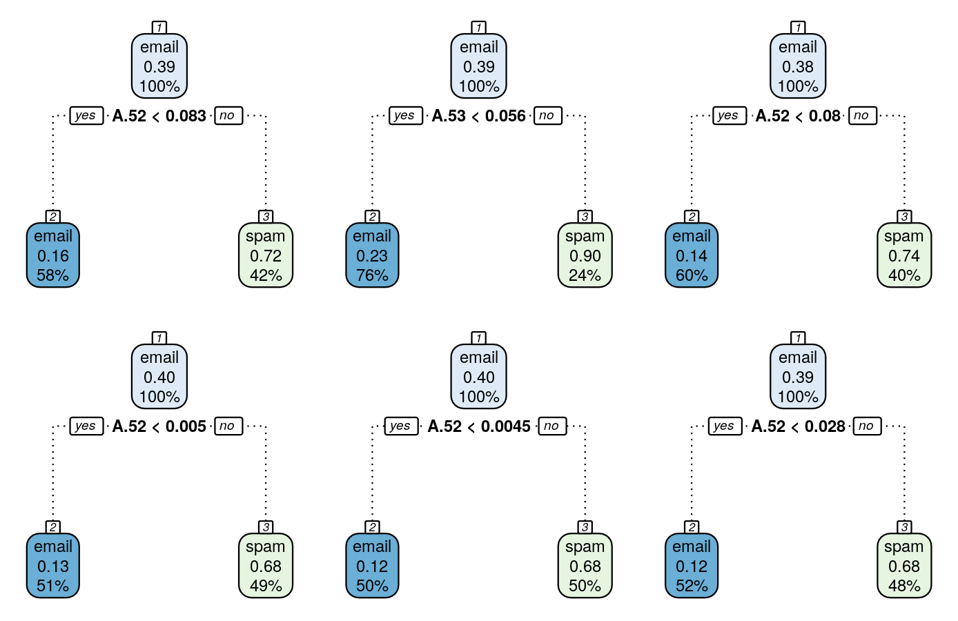
- 학습자료의 작은 변화에 의해 예측모형이 크게 변하는 경우에는 그 학습방법은 불안정(unstable)하다고 함. 아래는 동일한 데이터에서 랜덤추출한 자료를 학습자료로 이용하여 트리모형을 구축한 예시로 트리모형의 불안정성을 확인할 수 있음

- 앙상블방법
- 아래와 같이 여러개의 약한 기본모형(week base model, weak learner)을 결합하여 강한 모형(strong model)을 생성하고 이를 이용하여 예측, 단일모형의 불안정성(instability)을 극복하고 예측력을 향상하는 방법. 자주 사용하는 앙상블 모형은 배깅, 랜덤포레스트, 부스팅 등이 있음
\[ f(x) = \sum_{i=1}^M w_i f_i(x). \]

- 배깅(Bagging)
- 훈련데이터에서 랜덤하게 추출된 데이터를 이용하여 약한 의사결정나무모형을 만들어 각 트리모형의 예측치의 평균(회귀모형인 경우) 또는 다수결의 방법으로 결합하는 앙상블 방법으로 Breiman (1996)이 제안함

- 랜덤포레스트(Random Forest)
- 배깅방법에 비해 기본모형 생성시 더 많은 무작위성을 부여하는 방법으로 배깅방법과 유사하게 랜덤추출된 자료를 이용하나 기본 트리모형의 형성단계에서 랜덤하게 분리변수(split variable)와 분리값(split)을 선택함 Breiman (2001)이 제안함, 배깅의 일반화된 모형으로 볼 수 있으며, 예측력이 배깅보다 더 높고, 부스팅에 비해 과적합이 일어나지 않는다는 장점이 있음
- 부스팅(Boosting)
- 예측력이 약한 모형(weak learner)들을 결합하여 강한 예측모형을 만들기 위해 고안됨. 약한 예측모형이란 랜덤하게 예측하는 것보다 약간 좋은 예측력을 지닌 모형. 부스팅은 주어진 훈련자료에 대하여 순차적으로 기본모형을 생성하여 결합한 모형에서의 예측오차를 이용한 데이터 가중치를 조정하여 다음 기본모형을 형성, 그리고 모형의 가중치를 계산하여 결합하는 앙상블 모형으로 Fruend와 Shapire(1996)가 처음 제안함 데이터의 가중치는 오분류된 자료에 크게 잘 분류된 자료는 적게 부여하며, 기본모형의 가중치는 오분류율이 작을수록 크게 부여함

- 이후 Freidman이 제안한 Gradient Boosting과 XGBoost(Extreme Gradient Boosting)등 개선된 알고리즘이 출현함
- 특히 XGBoost는 Gradient Boosting에 Regularization을 도입하고 병렬계산을 지원하여 빠른 계산과 더불어 정확도의 향상을 가져옴
5.1 Ensemble R 패키지
| R패키지 | R 함수 | 설명 |
|---|---|---|
| ipred | bagging() | Bagging with rpart tree |
| randomForest | randomForest() | Random Forest 적합 |
| importance() | 변수중요도 | |
| varImpPlot() | 변수중요도 그림 | |
| partialPlot() | 부분의존도 그림(partial dependence plot) | |
| gbm | gbm() | Stochastic Gradient Boosting |
| gbm.perf() | 최적 부스팅 회수 = 트리모형의 개수 계산 | |
| summary.gbm() | 변수 중요도 계산 (relative influence of each variable) | |
| pretty.gbm.tree() | 모형에 포함된 트리모형 출력 | |
| xgboost | xgboost() | Extreme Gradient Boosting |
5.2 배깅 (bagging)
데이터의 분할
data(spam, package = "ElemStatLearn")
# sampling index of train data
tr.idx <- sample(nrow(spam), 0.7*nrow(spam))
배깅트리의 적합: 500개의 트리로 구성된 배깅모형을 적합
library(ipred) # 패키지 로딩
library(ROCR)
# fit bagging model with stump(2-nodes trees)
m.bag <- bagging(spam~., data=spam[tr.idx, ], nbagg=500, control=list(maxdepth=1))
names(m.bag)
## [1] "y"      "X"      "mtrees" "OOB"    "comb"   "call"
m.bag$mtrees[[1]]$btree # 첫번째 트리모형
##
## n= 3220
##
## node), split, n, loss, yval, (yprob)
##       * denotes terminal node
##
## 1) root 3220 1277 email (0.6034161 0.3965839)
##   2) A.52< 0.0805 1881  289 email (0.8463583 0.1536417) *
##   3) A.52>=0.0805 1339  351 spam (0.2621359 0.7378641) *
plot bagging trees
library(rpart.plot); par(mfrow=c(2,3))
for(i in 1:6){
  rpart.plot(m.bag$mtrees[[i]]$btree, branch.lty=3, nn=TRUE)
}
prediction & performance
pred_bag <- predict(m.bag, newdata=spam[-tr.idx, -58], type="prob")[,2] #class
( t_bag <- table(prediction=pred_bag>0.5, actural=spam$spam[-tr.idx]) )

##           actural
## prediction email spam
##      FALSE   781  223
##      TRUE     47  330

p_bag <- prediction(pred_bag, spam$spam[-tr.idx])
roc_bag <- performance(p_bag, measure = "tpr", x.measure = "fpr")
auc_bag <- round(performance(p_bag, measure = "auc")@y.values[[1]], 4)
plot(roc_bag, main=paste0("ROC of bigging (AUC=", auc_bag, ")"))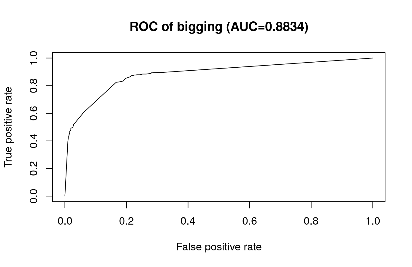
5.3 부스팅(boosting)
그래디언트부스팅 적합: 기본트리모형 500개 생성
library(gbm)
library(ROCR)
spam$spam <- as.integer(spam$spam=="spam")
gbm1 <- gbm(spam ~ ., data=spam[tr.idx, ], #var.monotone = c(0, 0, 0, 0, 0, 0),
        distribution = "bernoulli", #gaussian",
        n.trees = 500,
        #shrinkage = 0.1,
        #interaction.depth = 3,
        bag.fraction = 0.5, train.fraction = 0.5,
        n.minobsinnode = 10,
        cv.folds = 5, keep.data = TRUE,
        verbose = FALSE, n.cores = 1)
best.iter = gbm.perf(gbm1, method="cv")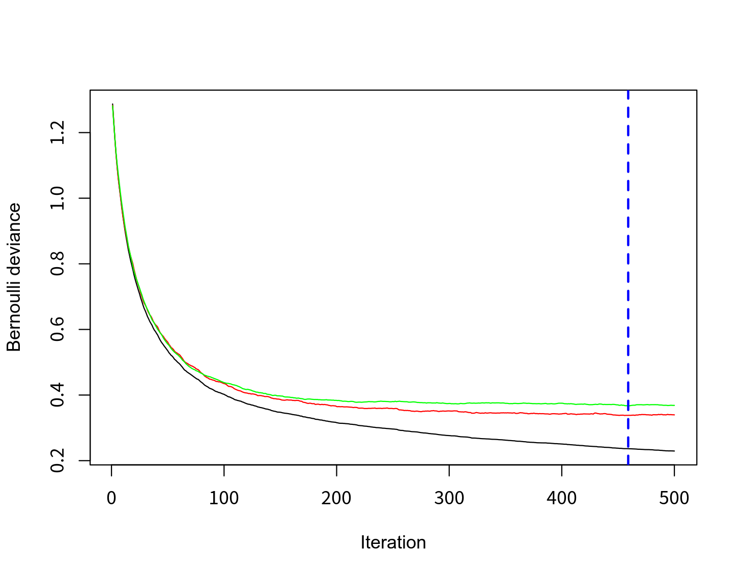
summary(gbm1)

##       var     rel.inf
## A.52 A.52 19.75124931
## A.53 A.53 13.98663217
## A.16 A.16 10.59330412
## A.7   A.7  9.98564280
## A.21 A.21  9.90696511
## A.25 A.25  7.13495475
## A.55 A.55  5.50060874
##    ...
## A.54 A.54  0.12666852
## A.20 A.20  0.11930810
## A.2   A.2  0.11891133
## A.6   A.6  0.08916727
## A.48 A.48  0.03854452
## A.44 A.44  0.03807381
##     ...
## A.47 A.47  0.00000000
## A.51 A.51  0.00000000
Plots the marginal effect of the selected variables by “integrating” out the other variables.
plot(pretty.gbm.tree(gbm1, i.tree = 6))boosting: prediction & performance
pred.boo <- predict(gbm1, newdata=spam[-tr.idx, -58], type="response") #link
( t_boo <- table(prediction=pred.boo>0.5, actural=spam$spam[-tr.idx]))

##           actural
## prediction   0   1
##      FALSE 804  54
##      TRUE   19 504

# Plot ROC
p_boo <- prediction(pred.boo, spam$spam[-tr.idx])
roc_boo <- performance(p_boo, measure = "tpr", x.measure = "fpr")
auc_boo <- round(performance(p_boo, measure = "auc")@y.values[[1]], 4)
plot(roc_boo, main=paste0("ROC of gbm (AUC=", auc_boo, ")"))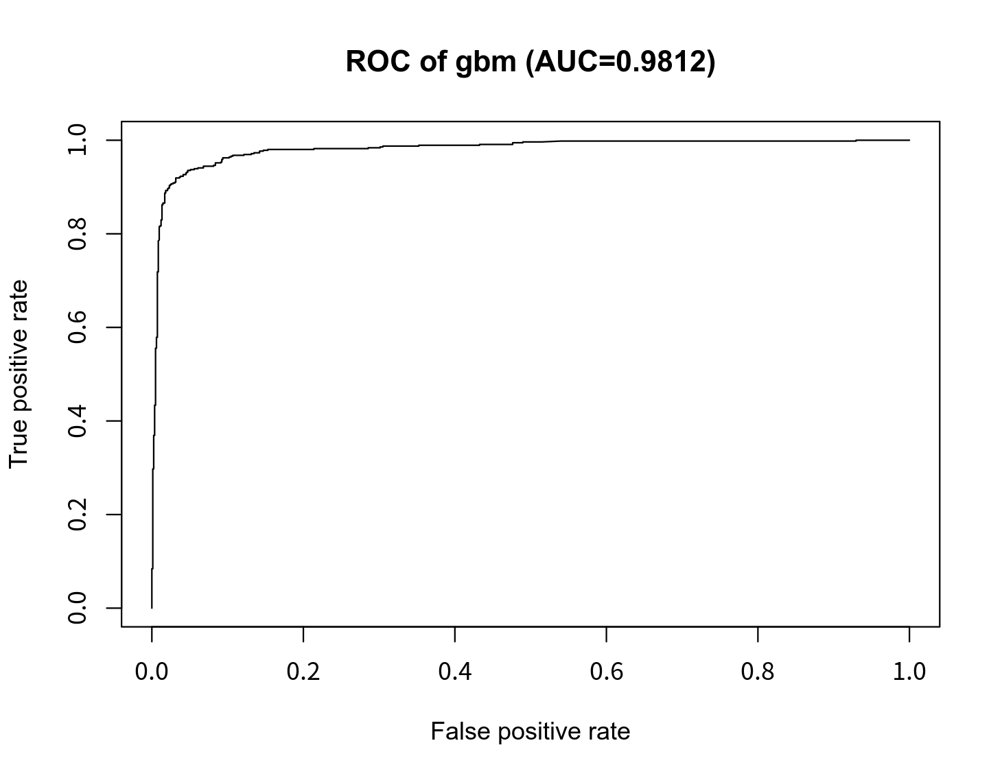
5.4 Random Forest (Breiman, 2001)
Node size in tree: 2 (stump)
Number of trees: 500
No. of candidate split variables: 2-5
모형적합: 기본트리모형(stump 이용), 변수중요도 계산 포함
library(randomForest); #require(rpart)
# fit RF model with stump(2-nodes trees)
spam$spam <- factor(spam$spam)
m.rf <- randomForest(x=spam[tr.idx, -58], y=spam$spam[tr.idx],
                     ntree=500, mtry=7,
                     importance=TRUE # 변수중요도
                     )
names(m.rf)
##  [1] "call"            "type"            "predicted"       "err.rate"        "confusion"       "votes"
##  [7] "oob.times"       "classes"         "importance"      "importanceSD"    "localImportance" "proximity"
## [13] "ntree"           "mtry"            "forest"          "y"               "test"            "inbag"
변수 중요도 시각화 (variables Importance plot)
# type=1: mean decrease in accuracy, 2:mean decrease in node impurity
varImpPlot(m.rf, type=1)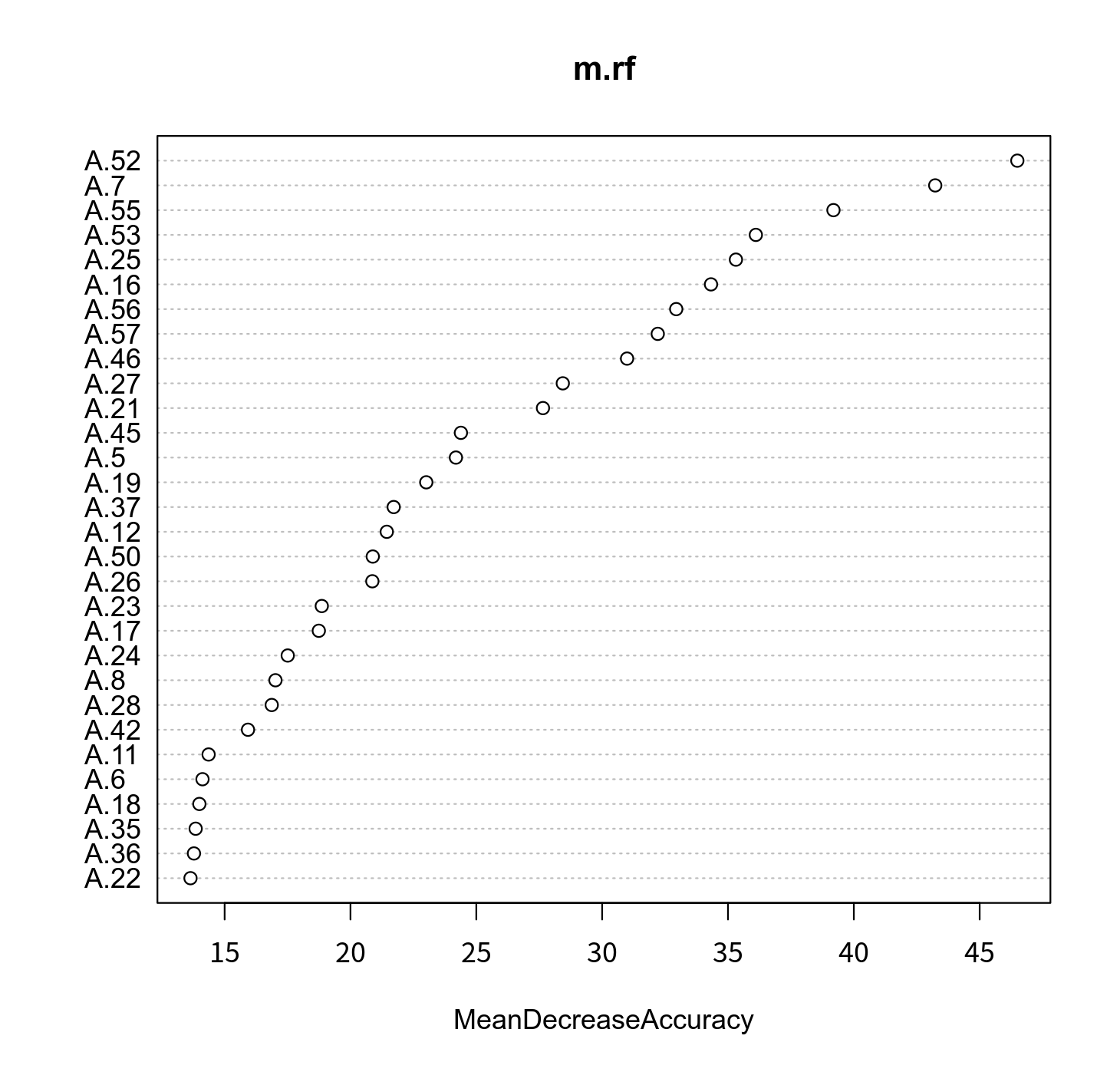
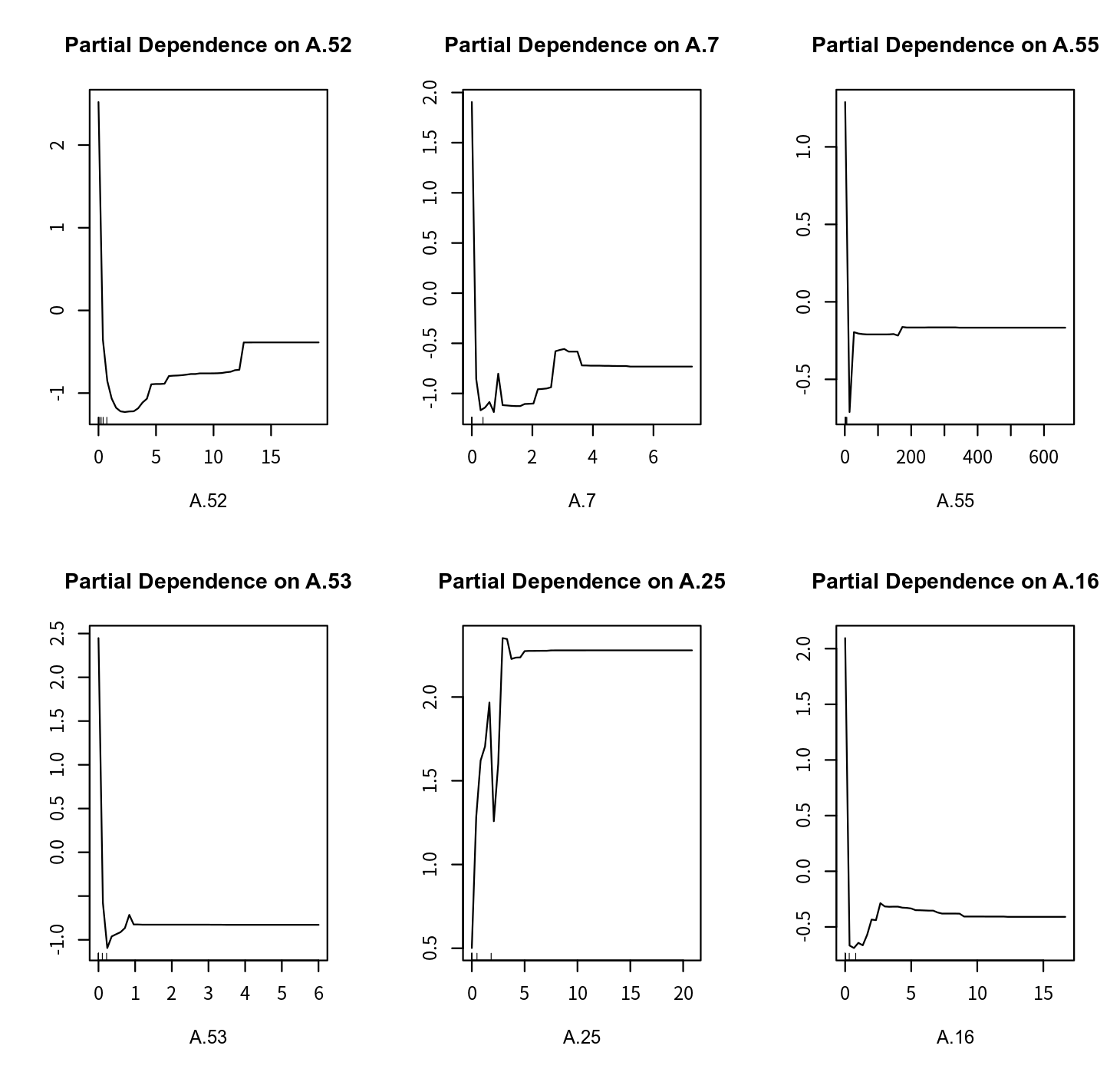
Partial dependence plot
partialPlot(x, pred.data, x.var)- x: rf model
- pred.data : training data
- x.var : variable name to be examined
imp <- importance(m.rf, type=1) # Mean Decrease Accuracy
impvar <- rownames(imp)[order(imp[, 1], decreasing=TRUE)]
par(mfrow=c(2, 3))
for (i in 1:6){
    partialPlot(m.rf, pred.data=spam[tr.idx,], impvar[i], xlab=impvar[i],
                main=paste("Partial Dependence on", impvar[i]))
}
prediction & performance
pred.rf <- predict(m.rf, newdata=spam[-tr.idx, -58], type="prob")[,2] #response|prob
(t_rf <- table(prediction=pred.rf>0.5, actural=spam$spam[-tr.idx]))
p_rf <- prediction(pred.rf, spam$spam[-tr.idx])
roc_rf <- performance(p_rf, measure = "tpr", x.measure = "fpr")
auc_rf <- round(performance(p_rf, measure = "auc")@y.values[[1]], 4)
plot(roc_rf, main=paste0("ROC of RF (AUC=", auc_rf, ")"))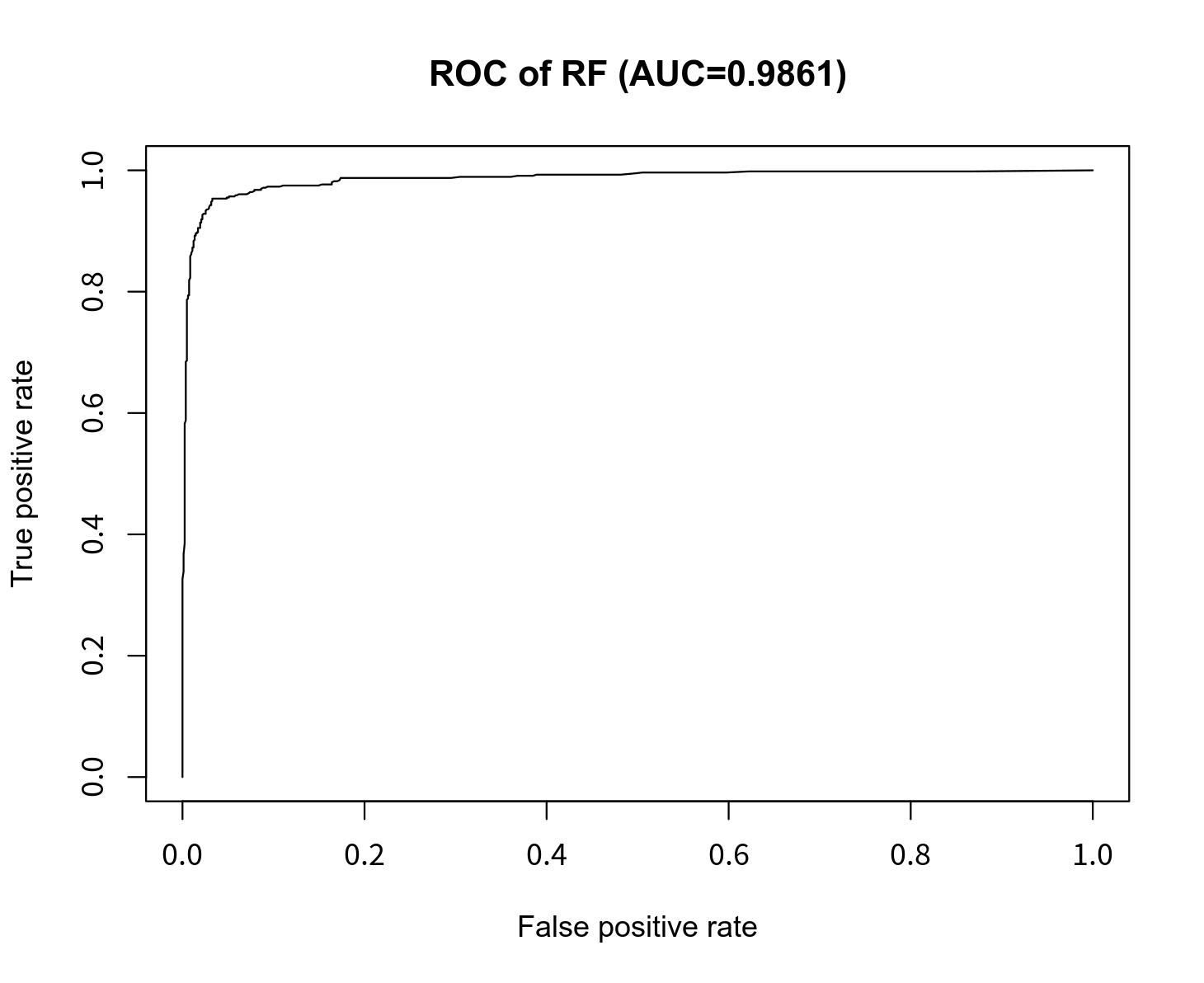
5.5 XGboost
XGboost모형 적합
library(xgboost)
data(agaricus.train, package='xgboost')
data(agaricus.test, package='xgboost')
train <- agaricus.train
test <- agaricus.test
bst <- xgboost(data = train$data, label = train$label, max_depth = 2, #eta = 1,
               nthread = 20,
               verbose = 0,
               nrounds = 2000, objective = "binary:logistic")
bst

## ##### xgb.Booster
## raw: 1.4 Mb
## call:
##   xgb.train(params = params, data = dtrain, nrounds = nrounds,
##     watchlist = watchlist, verbose = verbose, print_every_n = print_every_n,
##     early_stopping_rounds = early_stopping_rounds, maximize = maximize,
##     save_period = save_period, save_name = save_name, xgb_model = xgb_model,
##     callbacks = callbacks, max_depth = 2, nthread = 20, objective = "binary:logistic")
## params (as set within xgb.train):
##   max_depth = "2", nthread = "20", objective = "binary:logistic", validate_parameters = "TRUE"
## xgb.attributes:
##   niter
## callbacks:
##   cb.evaluation.log()
## # of features: 126
## niter: 2000
## nfeatures : 126
## evaluation_log:
##     iter train_logloss
##        1  0.4825405066
##        2  0.3595360332
## ---
##     1999  0.0004419146
##     2000  0.0004419146
예측
pred <- predict(bst, test$data)
prediction <- as.numeric(pred > 0.5)
table(prediction, test$label)

## prediction   0   1
##          0 835   0
##          1   0 776
입력변수의 중요도 (variable importances) 계산
importance_matrix <- xgb.importance(colnames(agaricus.train$data), model = bst)
xgb.plot.importance(importance_matrix,
                    top_n = 20,
                    rel_to_first = TRUE,
                    xlab = "Relative importance")
xgb.ggplot.importance(importance_matrix,
                    top_n = 20,
                    rel_to_first = TRUE,
                    xlab = "Relative importance")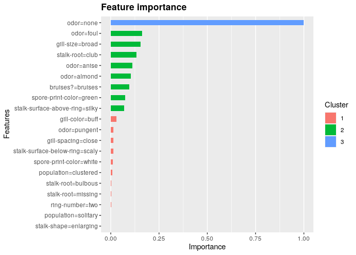
5.6 Comparison: bagging, boosting, RF
err <- c(sum(diag(t_bag))/sum(t_bag),
sum(diag(t_boo))/sum(t_boo),
sum(diag(t_rf))/sum(t_rf))
auc <- c(auc_bag, auc_boo, auc_rf)

p <- data.frame(`Error Rate`=err, `AUC`=auc)
rownames(p) <- c("bagging", "gbm", "Random Forest")
p

##               Error.Rate    AUC
## bagging        0.7740768 0.8649
## gbm            0.9456915 0.9823
## Random Forest  0.9543809 0.9847