제 7 장 딥러닝 기초 (DNN, Deep Neural Network)

7.1 필요 패키지 설치 및 로딩

반드시 버전 체크할 것 (낮은 버전은 업그레이드)

install.packages("tensorflow") # version 2.8.0
install.packages("keras")      # version 2.8.0
install.packages("AmesHousing")      # data

패키지 로딩
```
library("keras")
library(AmesHousing)
```
데이터 생성

# one hot encode --> we use model.matrix(...)[, -1] to discard the intercept
data_onehot <- model.matrix(~ ., make_ames())[, -1] %>% as.data.frame()

# Create training (70%) and test (30%) sets for the AmesHousing::make_ames() data.
# Use set.seed for reproducibility
set.seed(12345)
split <- rsample::initial_split(data_onehot, prop = .7, strata = "Sale_Price")
train <- rsample::training(split)
test  <- rsample::testing(split)

# Create & standardize feature sets
# training features
train_x <- train %>% dplyr::select(-Sale_Price)
mean_    <- colMeans(train_x)
std_     <- apply(train_x, 2, sd)

# 표준화
train_x <- scale(train_x, center = mean_, scale = std_)

# testing features
test_x <- test %>% dplyr::select(-Sale_Price)
test_x <- scale(test_x, center = mean_, scale = std_)

# Create & transform response sets
train_y <- log(train$Sale_Price)
test_y  <- log(test$Sale_Price)

# zero variance variables (after one hot encoded) cause NaN so we need to remove
zv <- which(colSums(is.na(train_x)) > 0, useNames = FALSE)
train_x <- train_x[, -zv]
test_x  <- test_x[, -zv]

# What is the dimension of our feature matrix?
dim(train_x)
## [1] 2049  299
dim(test_x)
## [1] 881 299

7.2 모델 아키텍처

# model <- keras_model_sequential() %>%
#   layer_dense(units = 10, input_shape = ncol(train_x)) %>%
#   layer_dense(units = 5) %>%
#   layer_dense(units = 1)
# 
# model <- keras_model_sequential() %>%
#   layer_dense(units = 10, activation = "relu", input_shape = ncol(train_x)) %>%
#   layer_dense(units = 5, activation = "relu") %>%
#   layer_dense(units = 1)

model <- keras_model_sequential() %>%
  # network architecture
  layer_dense(units = 10, activation = "relu", input_shape = ncol(train_x)) %>%
  layer_dense(units = 5, activation = "relu") %>%
  layer_dense(units = 1) %>%
  # backpropagation
  compile(
    optimizer = "rmsprop",
    loss = "mse",
    metrics = c("mae")
  )

model
##
## Layer (type)                              Output Shape                          Param #        
## ===============================================================================================
## dense_2 (Dense)                           (None, 10)                            3000           
## _______________________________________________________________________________________________
## dense_1 (Dense)                           (None, 5)                             55             
## _______________________________________________________________________________________________
## dense (Dense)                             (None, 1)                             6              
## ===============================================================================================
## Total params: 3,061
## Trainable params: 3,061
## Non-trainable params: 0
## _______________________________________________________________________________________________

7.3 Model training

fit(x, y, batch_size, epochs, validation_split, verbose)
- batch_size: 목적함수를 최적화하는 알고리즘(SGD) 반복 수행시 필요한 데이터의 크기 (default = 32)
- epochs: 알고리즘의 반복 수행 횟수, 알고리즘의 총 연산 횟수 = batch_size * epochs
- validation_split: cross-validation을 수행할 때 필요한 평가 데이터의 비율(0~1)로 입력자료를 훈련자료 _ 평가자료로 분리함
- verbose: 알고리즘 수행 중 중간 결과를 표시 (default = FALSE)

code example

# train our model
learn <- model %>% fit(
  x = train_x,
  y = train_y,
  epochs = 50,
  batch_size = 32,
  validation_split = .2,
  verbose = FALSE
)

learn

## Final epoch (plot to see history):
##     loss: 0.5952
##      mae: 0.2349
## val_loss: 6.512
##  val_mae: 1.109  
plot(learn)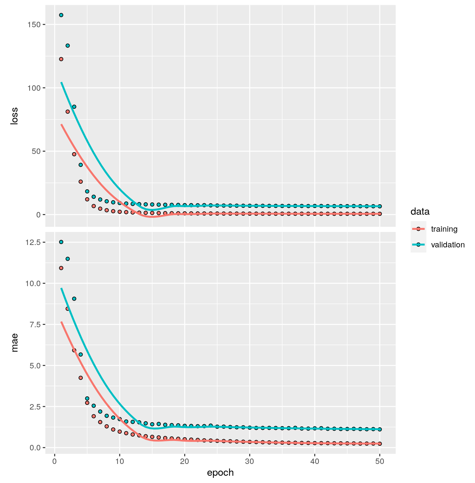

7.4 Model tuning

tuning process
1. 모형 구조 재설계 (layers & nodes)
2. Increase epochs if you do not see a flatlined loss function
3. Add batch normalization
4. Add dropout
5. Add weight regularization
6. Adjust learning rate

model <- keras_model_sequential() %>%
  # network architecture
  layer_dense(units = 20, activation = "relu", input_shape = ncol(train_x)) %>%
  layer_batch_normalization() %>%
  layer_dropout(rate = 0.2) %>%
  layer_dense(units = 5, activation = "relu") %>%
  layer_batch_normalization() %>%
  layer_dropout(rate = 0.2) %>%
  layer_dense(units = 1) %>%
  # backpropagation
  compile(
    optimizer = "rmsprop",
    loss = "mse",
    metrics = c("mae")
  )

model

# train our model
learn <- model %>% fit(
  x = train_x,
  y = train_y,
  epochs = 25,
  batch_size = 32,
  validation_split = .2,
  verbose = FALSE
)

plot(learn)