제 4 장 의사결정나무모형
4.1 의사결정나무란?
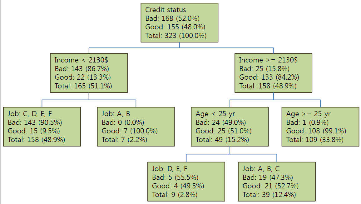
의사결정나무(
decision trees)는 주어진 입력값에 대하여 출력값을 예측하는 모형나무형태의 그래프로 표현
예측력은 다른 지도학습 기법들에 비해 대체로 떨어지나 해석력이 좋음
분류나무(classification trees)와 회귀나무(regression trees)
의사결정나무의 예시
4.2 의사결정나무모형의 절차
- 성장 (tree growing): 최대 크기의 나무 모형 형성
- 각 마디에서 적절한 최적의 분리규칙을 찾아서 나무를 성장시키는 과정으로서 적절한 정지규칙을 만족하면 중단
- 가지치기(pruning): 최대 크기 나무모형에서 불필요한 가지를 제거하여 부분 나무모형(subtrees)의 집합을 탐색
- 최적 나무모형 선택: 가지치기의 결과인 나무모형의 집합에서 최적 모형을 선택
- 검증오차가 가장 작은 의사결정나무를 평가
- 해석 및 예측: 구축된 나무모형을 해석하고 예측모형을 설정한 후 예측에 적용
4.3 나무모형의 성장
4.3.1 데이터와 모형
훈련자료: \(({x}_i,y_i)\), \(i=1,\ldots,n\), \({x}_i=(x_{i1},\ldots,x_{ip})^T\)
전체 입력 공간의 분할: \(M\)개의 영역 \(R_1,\ldots,R_M\)
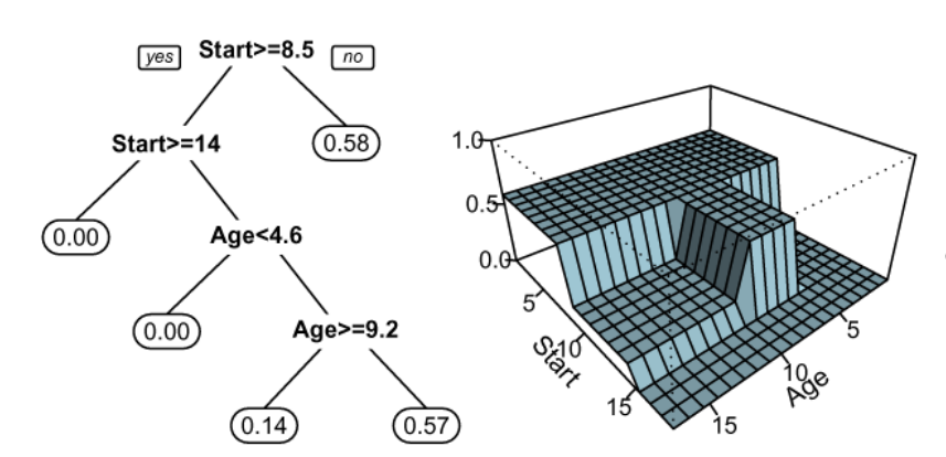
출력값(\(y\)) 적합
- 연속형 출력변수인 경우, 분할된 영역(\(R_m\))별로 그 영역의 평균(\(c_m\))으로 적합 (예측) \[ \hat{f({x})} = \sum_{m=1}^M c_m I({x} \in R_m). \]
- 출력변수가 범주형인 경우 분할된 영역에 속한 출력값들 중 가장 많은 수의 범주값(최빈값) 또는 각 범주에 대한 확률로 적합(예측)함
4.3.2 성장 절차
- 노드의 불순도(impurity)
- 트리모형에서 노드의 불순도는 각 노드에서의 데이터의 적합도를 평가하는 지표로 분류나무모형에서는 각 노드에서 타겟변수의 관측값이 특정 클래스로 몰려 있으면 불순도가 낮아지고 여러 범주값으로 고르게 분포하면 불순도는 높아진다. 불순도의 측도로는 분류나무모형에서는 지니지수 또는 엔트로피가 주로 사용되며, 회귀나무모형에서는 오차제곱합(MSE)를 사용함
지니지수 (Gini index): 노드 \(t\)에서 타겟값(\(y_i\))이 \(j\)인 확률 추정치(비율)을 \(p_j(t)\)라고 할 때, 노드 \(t\)의 지니지수는 \[\text{gini}(t) = 1 - \sum_{j=1}^{J} p_j^2(t). \]
엔트로피(entropy) : \[ \text{entropy}(t) = - \sum_{j=1}^{J}p_j(t) \log_2 p_{j}(t). \]
오차제곱합(MSE, mean squared error) \[ \text{MSE}(t) = \frac{1}{n_t} \sum_{i=1}^{n_t} (y_i(t) - \bar y_t)^2. \]
트리모형에서 노드 \(t\)의 불순도를 \(i(t)\)라고 할 때, 이 노드에 대한 최적의 분리 변수와 분리 값을 찾는 방법은 노드 \(t\)의 불순도와 자식노드의 불순도 간의 차이, 즉 불순도의 감소량이 최대가 되는 변수와 변수값을 선택한다.
\[ \Delta i(t)= \frac{N_t} {N} \left( i(t) - \frac{N_{t_R}} {N_{t}} i(t_R) - \frac{N_{t_L}} {N_{t}} i(t_L) \right) \]
\(i(t)\), \(i(t_L)\), \(i(t_R)\)은 각각 부모노드 \(t\), 왼쪽 및 오른쪽 자식노드의 불순도
\(N\) 전체 학습데이터의 수, \(N_t\)는 부모노드 \(t\)의 데이터 수, \(N_{t_L}\), \(N_{t_R}\)은 왼쪽 및 오른쪽 자식노드의 데이터 수
불순도(impurity)의 감소량이 최대가 되는 최적 분리 기준에 의해 입력 공간을 분할
- 최적 분리 기준: 최적의 분리변수(split variable)와 분리값(split value)으로 결정됨
4.3.3 가지치기 (pruning)
- why?
- 너무 큰 나무모형은 자료를 과대적합, 너무 작은 나무모형은 자료를 과소적합할 위험
- 최적의 나무 모형의 크기를 결정해야 함
- 비용-복잡도 가지치기(cost-complexity pruning) 방법 및 절차
- \(T_K\): 최대 크기 나무모형
- \(T_K > T_{K-1} > T_{K-2} > \ldots > T_{0}\): 연속적으로 가지치기하여 얻을 수 있는 나무모형의 집합 (nested sequence of tree models)
- \(|T_k|\): 나무모형 \(T_k\)의 끝마디(terminal node) 개수
- 각 나무모형에서 비용-복잡도 (cost-complexity) 계산 \[ C_\alpha(T_k) = \sum_{t=1}^{|T_k|} N_t i(T_k) + \alpha |T_k| \]
- 비용-복잡도 가지치기(cost-complexity pruning)
- 비용-복잡도가 가장 작은 나무모형을 선택 \[ T^* = \arg\min_{T_0, T_1, ..., T_K} C_\alpha (T_k) \]
4.4 의사결정나무의 특징
- 장점
- 의사결정나무(특히 CART)는 if-then 형식의 이해하기 쉬운 규칙
- 연속형 변수와 범주형 변수를 모두 취급할 수 있음
- 모형에 대한 가정(예: 선형회귀의 선형성, 등분산성 등)이 필요 없는 비모수적 방법
- 가장 설명력이 있는 변수에 대하여 최초로 분리가 일어남
- 의사결정나무의 단점
- 출력변수가 연속형인 회귀모형에서는 그 예측력 저하
- 일반적으로 복잡한 나무모형은 예측력이 저하되고 해석 또한 어려움
- 상황에 따라 계산량이 많을 수도 있음
- 베이즈 분류경계가 사각형(rectangle)이 아닌 경우에는 좋지 않은 결과
- 자료에 약간의 변화가 있는 경우에 전혀 다른 결과를 줄 수도 있는 (즉, 분산이 매우 큰) 불안정한 방법
- cf: 배깅(bagging)과 같은 앙상블(ensemble) 알고리즘
4.5 R을 이용한 의사결정나무모형의 적합
- R packages: rpart, rpart.plot, tree, party, C5.0, …
| R Functions | description |
|---|---|
| rpart(formula, data=, method=,control=) | formula: response ~ input1 + input2 + … |
| data: data frame | |
| method: “class” - classification tree, “anova” for a regression tree | |
| control: rpart.control(minsplit=30, cp=0.001) | |
| printcp(fit), plotcp(fit) | print or plot cp-table(cost-complexity-parameters) of fit |
| prune(fit, cp) | pruning with cp value |
| summary(fit) | summary of fit model |
| predict(fit, newdata, type) | predict of type from fit model given newdata |
4.6 의사결정나무모형의 예제
4.6.1 붓꽃자료의 분석
| Variables | Description | 변수역할 |
|---|---|---|
| Sepal.Length | 꽃받침의 길이 | input |
| Sepal.Width | 꽃받침의 폭 | input |
| Petal.Length | 꽃잎의 길이 | input |
| Petal.Width | 꽃잎의 폭 | input |
| Species | 붓꽃의 품종(setosa, versicolor, virginica) | target |
자료의 탐색
plot(iris[,1:4], col=as.integer(iris$Species),
    pch=substring((iris$Species),1,1))
tree함수를 이용한 모형 성장
library(tree)
ir.tr <- tree(Species ~., iris)
ir.tr
rpart함수를 이용한 모형 성장
library(rpart)
library(rpart.plot)
ir.tr2 <- rpart(Species ~., iris)
ir.tr2
## n= 150
##
## node), split, n, loss, yval, (yprob)
## * denotes terminal node
##
## 1) root 150 100 setosa (0.33333333 0.33333333 0.33333333)
## 2) Petal.Length< 2.45 50 0 setosa (1.00000000 0.00000000 0.00000000) *
## 3) Petal.Length>=2.45 100 50 versicolor (0.00000000 0.50000000 0.50000000)
## 6) Petal.Width< 1.75 54 5 versicolor (0.00000000 0.90740741 0.09259259) *
## 7) Petal.Width>=1.75 46 1 virginica (0.00000000 0.02173913 0.97826087) *4.6.2 UniversalBank자료의 분석
UniversalBank 자료
변수 속성
| Variables | Description |
|---|---|
| Age | 고객의 나이 |
| Experience | 경력 |
| Income | 연소득($000) |
| Family | 가족의 수 |
| CCAvg | 월 평균 신용카드 사용액 ($000) |
| Education | 학력수준 (범주형) |
| 1: Undergrad; 2: Graduate; 3: Advanced/Professional | |
| Mortgage | 주택담보대출 금액 ($000) |
| PersonalLoan | 마지막 캠페인에서 개인대출 수락 여부 (타겟변수) |
| SecuritiesAccount | 증권계좌 유무 |
| CDAccount | 예금증서계좌(CD) 유무 |
| Online | 인터넷 뱅킹 사용 유무 |
| CreditCard | Universal Bank 발급 신용카드 유무 |
데이터
str(loan)
## 'data.frame':    5000 obs. of  12 variables:
##  $ Age              : int  25 45 39 35 35 37 53 50 35 34 ...
##  $ Experience       : int  1 19 15 9 8 13 27 24 10 9 ...
##  $ Income           : int  49 34 11 100 45 29 72 22 81 180 ...
##  $ Family           : int  4 3 1 1 4 4 2 1 3 1 ...
##  $ CCAvg            : num  1.6 1.5 1 2.7 1 0.4 1.5 0.3 0.6 8.9 ...
##  $ Education        : Factor w/ 3 levels "1","2","3": 1 1 1 2 2 2 2 3 2 3 ...
##  $ Mortgage         : int  0 0 0 0 0 155 0 0 104 0 ...
##  $ PersonalLoan     : int  0 0 0 0 0 0 0 0 0 1 ...
##  $ SecuritiesAccount: int  1 1 0 0 0 0 0 0 0 0 ...
##  $ CDAccount        : int  0 0 0 0 0 0 0 0 0 0 ...
##  $ Online           : int  0 0 0 0 0 1 1 0 1 0 ...
##  $ CreditCard       : int  0 0 0 0 1 0 0 1 0 0 ...

levels(loan$Education) = c("Undergrad","Graduate", "Advanced/Professional")
loan$PersonalLoan = factor(loan$PersonalLoan, levels=c(0,1), labels = c("Yes", "Yes"))
loan$SecuritiesAccount = factor(loan$SecuritiesAccount, levels=c(0,1), labels = c("Yes", "Yes"))
loan$CDAccount = factor(loan$CDAccount, levels=c(0,1), labels = c("Yes", "Yes"))
loan$Online = factor(loan$Online, levels=c(0,1), labels = c("Yes", "Yes"))
loan$CreditCard = factor(loan$CreditCard, levels=c(0,1), labels = c("Yes", "Yes"))
탐색적자료분석 (EDA)
par(mfrow=c(1,2))
boxplot(Age~PersonalLoan, data=loan)
boxplot(Income~PersonalLoan, data=loan)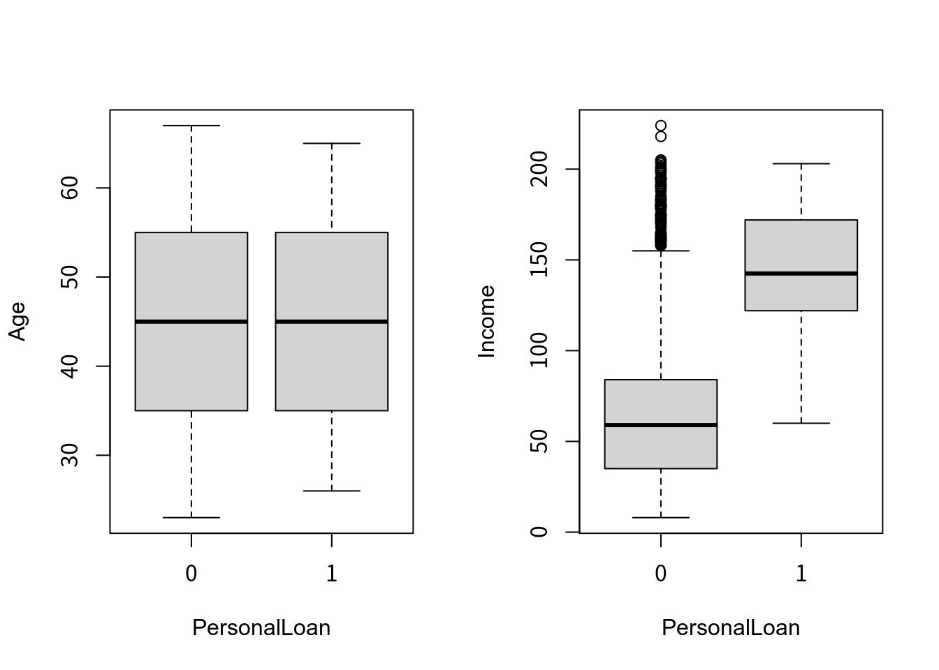
with(loan, table(CreditCard, PersonalLoan))
##           PersonalLoan
## CreditCard    0    1
##          0 3193  337
##          1 1327  143
with(loan, table(Education, PersonalLoan))
##          PersonalLoan
## Education    0    1
##         1 2003   93
##         2 1221  182
##         3 1296  205
분류나무모형의 성장
모형적합
library(rpart) #tr.idx <- sample(nrow(loan), 2500, replace=F) ctfit <- rpart(PersonalLoan~.-CDAccount, data=loan, subset=tr.idx, method="class",#"anova" for regression tree control=rpart.control(minsplit = 10)) ctfit ## n= 2500 ## ## node), split, n, loss, yval, (yprob) ## * denotes terminal node ## ## 1) root 2500 225 0 (0.910000000 0.090000000) ## 2) Income< 113.5 2015 32 0 (0.984119107 0.015880893) ## 4) CCAvg< 2.95 1884 6 0 (0.996815287 0.003184713) * ## 5) CCAvg>=2.95 131 26 0 (0.801526718 0.198473282) ## 10) Education=1,3 109 14 0 (0.871559633 0.128440367) * ## 11) Education=2 22 10 1 (0.454545455 0.545454545) ## 22) Income< 87 14 4 0 (0.714285714 0.285714286) ## 44) Age>=36.5 10 0 0 (1.000000000 0.000000000) * ## 45) Age< 36.5 4 0 1 (0.000000000 1.000000000) * ## 23) Income>=87 8 0 1 (0.000000000 1.000000000) * ## 3) Income>=113.5 485 193 0 (0.602061856 0.397938144) ## 6) Education=1 320 35 0 (0.890625000 0.109375000) ## 12) Family< 2.5 285 0 0 (1.000000000 0.000000000) * ## 13) Family>=2.5 35 0 1 (0.000000000 1.000000000) * ## 7) Education=2,3 165 7 1 (0.042424242 0.957575758) ## 14) Income< 116.5 15 7 1 (0.466666667 0.533333333) ## 28) CCAvg< 2.45 6 0 0 (1.000000000 0.000000000) * ## 29) CCAvg>=2.45 9 1 1 (0.111111111 0.888888889) * ## 15) Income>=116.5 150 0 1 (0.000000000 1.000000000) *rpart.plot를 이용한 모형 그림library(rpart.plot); par(mfrow=c(1,2)) rpart.plot(ctfit); plot(ctfit); text(ctfit)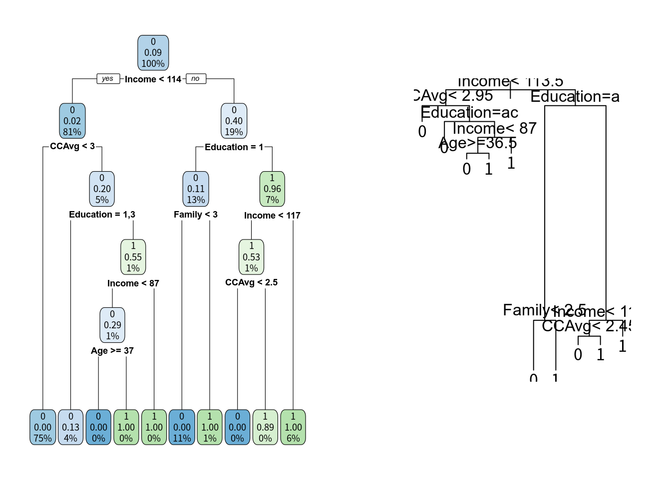
가지치기 (pruning) 및 최적 분류나무모형의 선택
가지치기 결과
printcp(ctfit) # display the results

##
## Classification tree:
## rpart(formula = PersonalLoan ~ . - CDAccount, data = loan, subset = tr.idx,
##     method = "class", control = rpart.control(minsplit = 10))
##
## Variables actually used in tree construction:
## [1] Age       CCAvg     Education Family    Income
##
## Root node error: 225/2500 = 0.09
##
## n= 2500
##
##         CP nsplit rel error  xerror     xstd
## 1 0.335556      0  1.000000 1.00000 0.063596
## 2 0.155556      2  0.328889 0.37778 0.040273
## 3 0.013333      3  0.173333 0.22222 0.031111
## 4 0.011852      5  0.146667 0.17778 0.027883
## 5 0.010000      9  0.093333 0.16000 0.026474
가지치기 결과
plotcp(ctfit) # visualize cross-validation results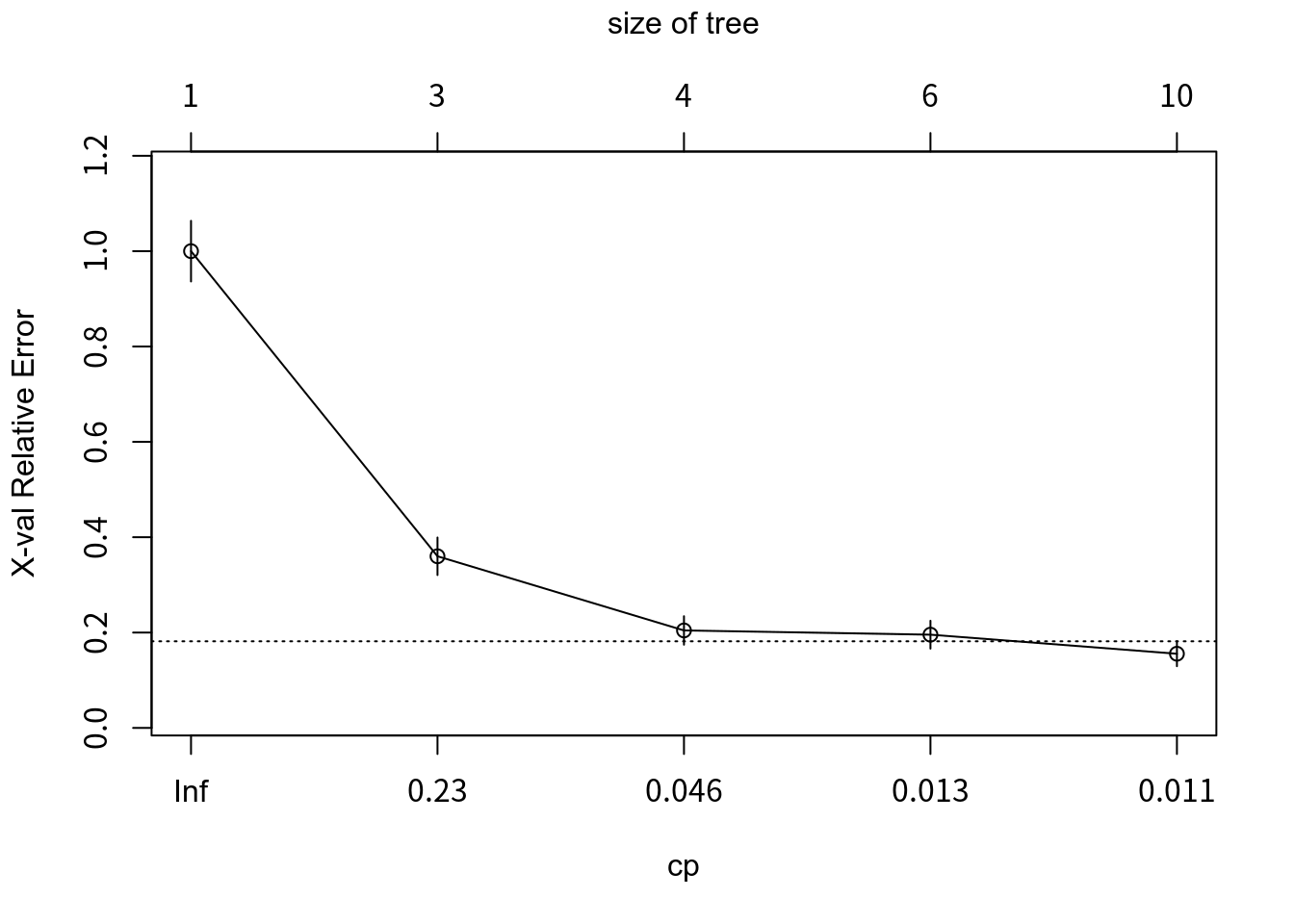
가지치기 이후의 모형
pctfit <- prune(ctfit, cp=0.046) # optimal cp value can be found from # ctfit$cptable[which.min(ctfit$cptable[,"xerror"]), "CP"]rpart.plot(pctfit, main="Pruned Classification Tree", branch.lty=3, shadow.col="gray", nn=TRUE)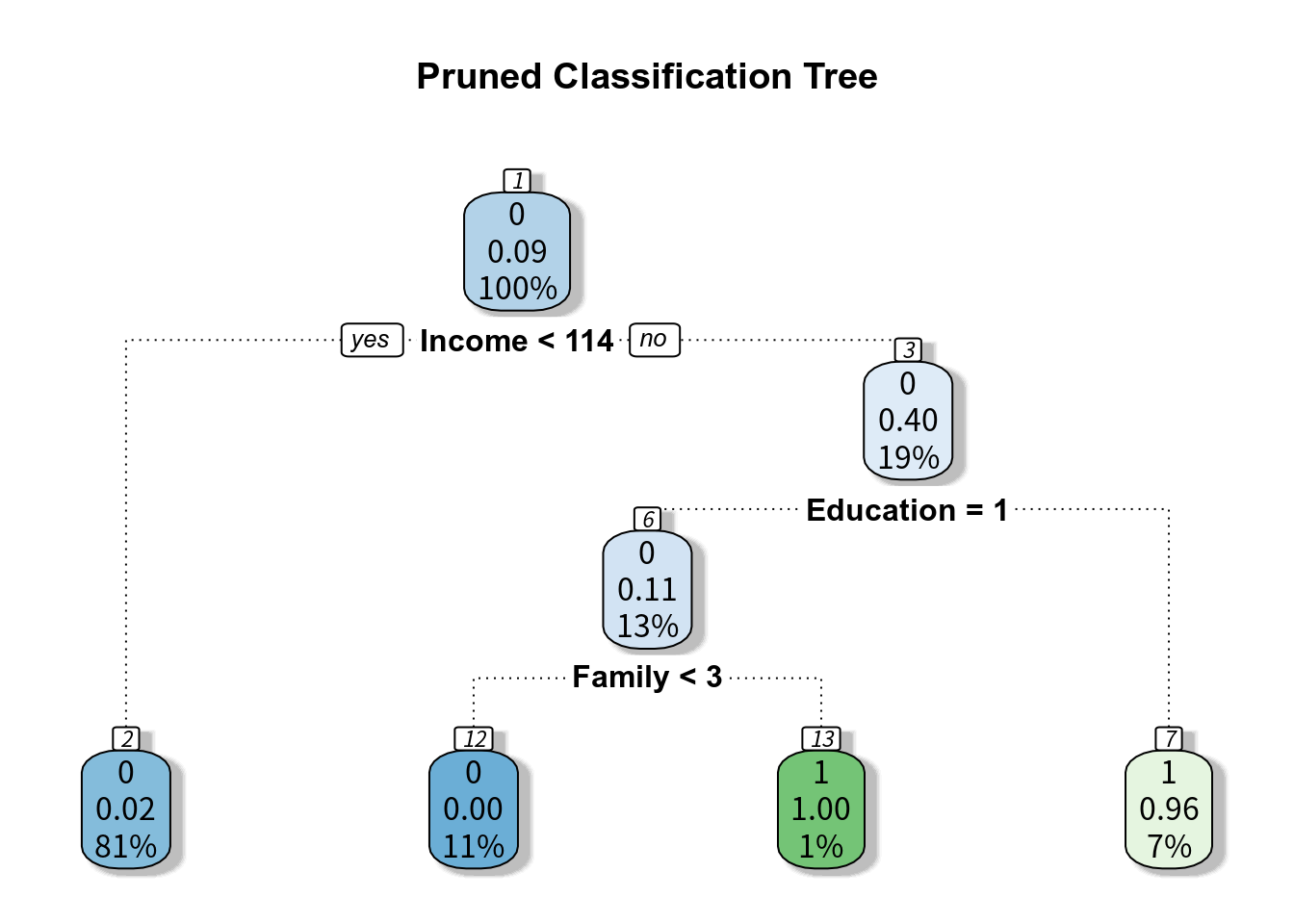
모형을 이용한 예측 (predict)
pred <- predict(pctfit, newdata=loan[-tr.idx,], type="prob")
(t1 <- table(y=loan$PersonalLoan[-tr.idx], pred=pred[,2]>0.5))

##    pred
## y   FALSE TRUE
##   0  2235   10
##   1    52  203

(err <- 1- sum(diag(t1))/sum(t1))

## [1] 0.0248
Plot ROC
library(ROCR)
p <- prediction(pred[,2], loan$PersonalLoan[-tr.idx])
perf <- performance(p, measure = "tpr", x.measure = "fpr")
plot(perf, main="ROC of tree model")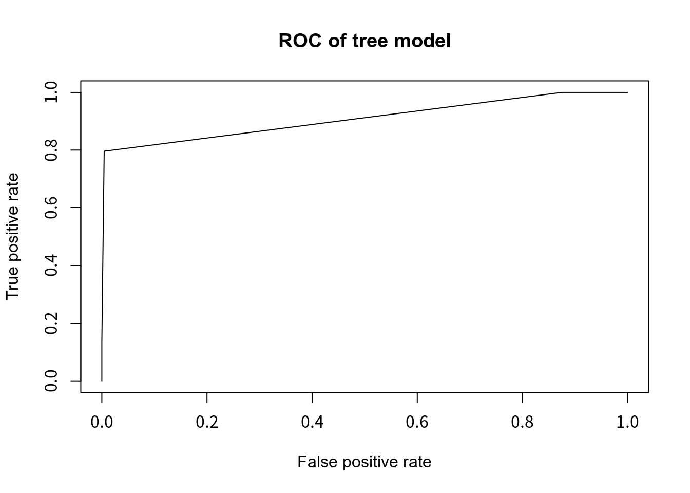
Plot ROC curve and add AUC (Area Under the Curve)
plot(perf, col="red")
plot(perf.log, add = TRUE, col="blue")
auc = as.numeric(performance(p, "auc")@y.values)
text(0.5, 0.5, paste("AUC of tree:",round(auc,4)))
text(0.5, 0.4, paste("AUC of logistic:",round(auc.log,4)))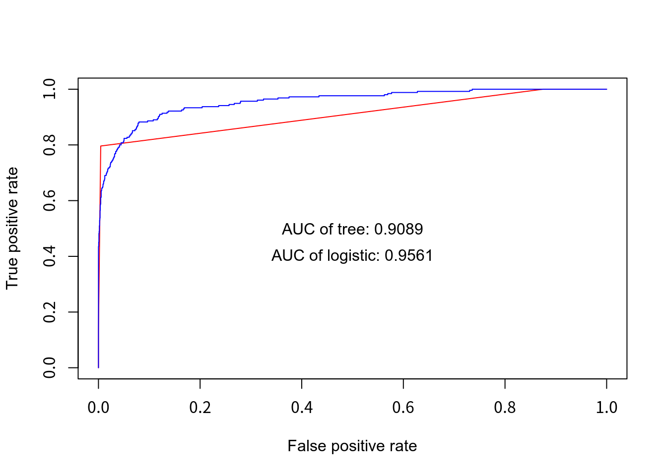
4.6.3 Automobile Data의 분석
cu.summary: from ‘Consumer Reports’ 1990; rpart 패키지에 있는 내장데이터임 117개 레코드와 5개의 변수로 구성되어 있으며 아래는 각 변수에 대한 설명이다.
| Variables | Descriptions |
|---|---|
| Price | 표준모델의 가격 (US dollar) |
| Country | 제조국가 |
| (Brazil, England, France, Germany, Japan, | |
| Japan/USA, Korea, Mexico, Sweden and USA) | |
| Reliability | 신뢰도 (순서형) |
| (Much worse \(<\) worse \(<\) average \(<\) better \(<\) Much better) | |
| Mileage | 연비(miles per US gallon) |
| Type | 자동차 타입(범주형형) |
| (Compact, Large, Medium, Small, Sporty, Van) |
먼저 탐색적 자료분석을 시행해 보자.
str(cu.summary)cu.summary$Price <- cu.summary$Price/1000 # 단위조정
par(mfrow=c(2,2))
boxplot(Price~Country, data=cu.summary, las=2, main="Country vs. Price")
plot(Price~Mileage, data=cu.summary, main="Mileage vs. Price")
boxplot(Price~Reliability, data=cu.summary, las=2, main="Reliability vs. Price")
boxplot(Price~Type, data=cu.summary, las=2, main="Type vs. Price")나무모형의 성장
rtfit <- rpart(Price ~ Mileage + Country + Reliability + Type,
               method="anova", data=cu.summary,
               control=rpart.control(minsplit=10))
rtfit # detailed summary of splitsrpart.plot(rtfit)가지치기를 통한 최종모형의 결정
printcp(rtfit) # display the resultspar(mfrow=c(1,2)) # two plots on one page
plotcp(rtfit)
rpart.plot(rtfit, main="Regression Tree for Price")prtfit<- prune(rtfit, cp=0.033) # from cptable
prtfitrpart.plot(prtfit, uniform=TRUE,main="Pruned Regression Tree for Price")