4 장 Numpy

4.1 NumPy(넘파이) 특징

과학 계산을 위한 라이브러리
행렬/배열 처리 및 연산
난수생성

4.2 배열의 생성

리스트에서 행렬/배열 생성

import numpy as np # numpy 패키지 로드하여 np로 사용
a = [[1,2,3], [4,5,6]] # 리스트에서 행렬생성
b = np.array(a) 
print(b)

## [[1 2 3]
##  [4 5 6]]

print(b.ndim)  # 배열의 열수(차원)

## 2

print(b.shape) # 배열의 차원

## (2, 3)

print(b[0,0])  # 배열의 원소 접근

## 1

특수한 배열의 생성

print(np.arange(10)) # 1씩 증가하는 1차원 배열(시작이 0부터)

## [0 1 2 3 4 5 6 7 8 9]

print(np.arange(5, 10)) # 1씩 증가하는 1차원 배열(시작이 5부터)

## [5 6 7 8 9]

print(np.zeros((2,2)))  # 영행렬 생성

## [[0. 0.]
##  [0. 0.]]

print(np.ones((2,3)))  # 유닛행렬

## [[1. 1. 1.]
##  [1. 1. 1.]]

print(np.full((2,3), 5)) # 모든 원소가 5인 2*3행렬

## [[5 5 5]
##  [5 5 5]]

print(np.eye(3)) # 단위행렬

## [[1. 0. 0.]
##  [0. 1. 0.]
##  [0. 0. 1.]]

배열의 차원 변환

a = np.arange(20)
print(a)

## [ 0  1  2  3  4  5  6  7  8  9 10 11 12 13 14 15 16 17 18 19]

b=a.reshape((4,5))
print(b)

## [[ 0  1  2  3  4]
##  [ 5  6  7  8  9]
##  [10 11 12 13 14]
##  [15 16 17 18 19]]

4.3 Numpy 슬라이싱/인덱싱

import numpy as np
lst = [
    [1, 2, 3],
    [4, 5, 6],
    [7, 8, 9]
]
arr = np.array(lst)
a = arr[0:2, 0:2]
print(a)

## [[1 2]
##  [4 5]]

a = arr[1:, 1:]
print(a)

## [[5 6]
##  [8 9]]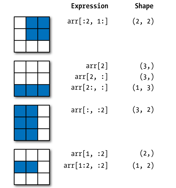

Two-dimensional array slicing

4.4 Numpy 연산

배열간 연산 가능
+,-,*,/ 등의 연산자 사용가능

add(),substract(),multiply(),divide()

import numpy as np

a = np.array([1,2,3])
b = np.array([4,5,6])

# 각 요소 더하기
c = a+b

# c= np.add(a, b)
print(c) # [-3 -3 -3]

# 각 요소 곱하기
# c = a*b

## [5 7 9]

c = np.multiply(a, b)
print(c) #[4 10 18]

# 각 요소 나누기
# c = a/b

## [ 4 10 18]

c = np.divide(a,b)
print(c) # [0.25 0.4 0.5]

## [0.25 0.4  0.5 ]

dot()함수: 행렬의 곱

import numpy as np
arr1 = [[1,2],[3,4]]
arr2 = [[5,6],[7,8]]
a = np.array(arr1)
b = np.array(arr2)

c= np.dot(a, b)
print(c)

## [[19 22]
##  [43 50]]

모든 원소의 합: sum(), 모든 원소의 곱: prod()

import numpy as np

a = np.array([[-1,2,3],[3,4,8]])
s = np.sum(a)
print('sum=',a.sum()) 

# 행별/열별 연산 (axis=0/1)

## sum= 19

print('sum by row=',a.sum(axis=0))

## sum by row= [ 2  6 11]

print('mean=',a.mean())

## mean= 3.1666666666666665

print('sd=',a.std())

## sd= 2.6718699236469

print('product=',a.prod())

## product= -576

4.5 기본 수학함수

Function	Description
abs, fabs	absolute value element-wise for integer, foating-point, or complex values
sqrt	square root of each element (equivalent to arr ** 0.5)
square	square of each element (equivalent to arr ** 2)
exp	exponent \(e^x\) of each element
log, log10,	Natural logarithm (base e), log base 10, log base 2, and log(1 + x), respectively
log2, log1p
sign	sign of each element: 1 (positive), 0 (zero), or –1 (negative)
ceil	ceiling of each element (i.e., 주어진 수보다 크거나 같은 최소 정수)
floor	floor of each element (i.e., 작거나 같은 최대정수)
rint	반올림
isnan	NaN (Not a Number) 체크, [True\|False]
isfinite, isinf	유한/무한 체크
cos, cosh, sin,	삼각함수
sinh, tan, tanh
arccos, arccosh,
arcsin, arcsinh,
arctan, arctanh

4.6 선형대수(벡터/행렬연산) 함수

Function	Description
diag	diagonal elements of a square matrix as a 1D array, or
	convert a 1D array into a square matrix with zeros on the off-diagonal
dot	Matrix multiplication
trace	sum of the diagonal elements
det	matrix determinant
eig	eigenvalues and eigenvectors of a square matrix
inv	inverse of a square matrix
pinv	Moore-Penrose pseudo-inverse of a matrix
qr	QR decomposition
svd	singular value decomposition (SVD)
solve	\(Ax = b\) for \(x\), where \(A\) is a matrix
lstsq	least-squares solution to \(Ax = b\)

벡터연산(내적) \[ \mathbf{x} = (1 , 2 , 3)', \mathbf{y} = (6, 23,-1)', \Rightarrow \mathbf{x}'\mathbf{y} = 1\times 6 + 2\times 23 + 3 \times (-1) = ? \]

import numpy as np
x = np.array([1, 2, 3])
print(x)

## [1 2 3]

y = np.array([6, 23,-1])
print(y)

## [ 6 23 -1]

print(x.dot(y.T) )# x'y

## 49

print(x.T.dot(y) )# x'y

## 49

\[ X = \begin{pmatrix} 1 & 2 & 3\\ 4 & 5 & 6 \end{pmatrix}, Y = \begin{pmatrix} 6 & 23\\ -1 & 7\\ 8 & 9 \end{pmatrix}\Rightarrow XY = ? \]

import numpy as np
x = np.array([[1., 2., 3.], [4., 5., 6.]])
y = np.array([[6., 23.], [-1, 7], [8, 9]])
print(x)

## [[1. 2. 3.]
##  [4. 5. 6.]]

print(y)

## [[ 6. 23.]
##  [-1.  7.]
##  [ 8.  9.]]

print(x.dot(y)) # xy

## [[ 28.  64.]
##  [ 67. 181.]]

print(y.dot(x)) # yx

## [[ 98. 127. 156.]
##  [ 27.  33.  39.]
##  [ 44.  61.  78.]]

역행렬

import numpy as np
from numpy.linalg import inv
np.random.seed()
X = np.array([[1,2,3],[1,0,0],[0,0,1]])
print(X)

## [[1 2 3]
##  [1 0 0]
##  [0 0 1]]

Y = inv(X)
print(Y)

## [[ 0.   1.   0. ]
##  [ 0.5 -0.5 -1.5]
##  [ 0.   0.   1. ]]

X.dot(Y)

## array([[1., 0., 0.],
##        [0., 1., 0.],
##        [0., 0., 1.]])

4.7 난수(랜덤넘버)의 생성

함수	분포
beta(a, b[, size])	Beta distribution.
binomial(n, p[, size])	binomial distribution.
chisquare(df[, size])	chi-square distribution.
exponential([scale, size])	exponential distribution.
f(dfnum, dfden[, size])	F distribution.
gamma(shape[, scale, size])	Gamma distribution.
geometric(p[, size])	geometric distribution.
hypergeometric(ngood, nbad,	Hypergeometric distribution.
nsample[, size])
multinomial(n, pvals[, size])	multinomial distribution.
negative_binomial(n, p[, size])	negative binomial distribution.
normal([loc, scale, size])	normal (Gaussian) distribution.
poisson([lam, size])	Poisson distribution.

균등분포에서 난수생성

x = np.random.uniform(size=100)
x.reshape(20,5)

## array([[0.62283254, 0.83247702, 0.69284631, 0.36343642, 0.1194816 ],
##        [0.95766884, 0.96097382, 0.82350006, 0.11160819, 0.54375729],
##        [0.24869946, 0.92595691, 0.99723618, 0.99178697, 0.23498384],
##        [0.39983813, 0.32569314, 0.7650107 , 0.61846918, 0.36615931],
##        [0.48812842, 0.78436822, 0.68059491, 0.17950023, 0.888353  ],
##        [0.64016348, 0.70486181, 0.14406225, 0.67690893, 0.43506099],
##        [0.89071105, 0.477524  , 0.42140245, 0.0449729 , 0.3284721 ],
##        [0.08859325, 0.44517624, 0.03226408, 0.9500857 , 0.79906355],
##        [0.24693298, 0.93577942, 0.4421043 , 0.82808844, 0.83521711],
##        [0.43705478, 0.35683298, 0.24488695, 0.91222773, 0.1276007 ],
##        [0.94680193, 0.8077273 , 0.45796358, 0.86975714, 0.52794646],
##        [0.21696068, 0.36560811, 0.4285624 , 0.57030412, 0.46012208],
##        [0.85012542, 0.30934787, 0.45566465, 0.39913531, 0.21541012],
##        [0.72966978, 0.62645567, 0.18330374, 0.34446564, 0.64710839],
##        [0.9289908 , 0.05556862, 0.03368774, 0.42573986, 0.44694258],
##        [0.1867547 , 0.68780933, 0.44845544, 0.08709105, 0.99633162],
##        [0.82920243, 0.6960733 , 0.89147693, 0.79821622, 0.11935229],
##        [0.44458672, 0.665925  , 0.11769361, 0.57772073, 0.20383055],
##        [0.34587712, 0.14346508, 0.97603253, 0.99795754, 0.89759219],
##        [0.62642511, 0.98741594, 0.77529789, 0.04090993, 0.68038324]])

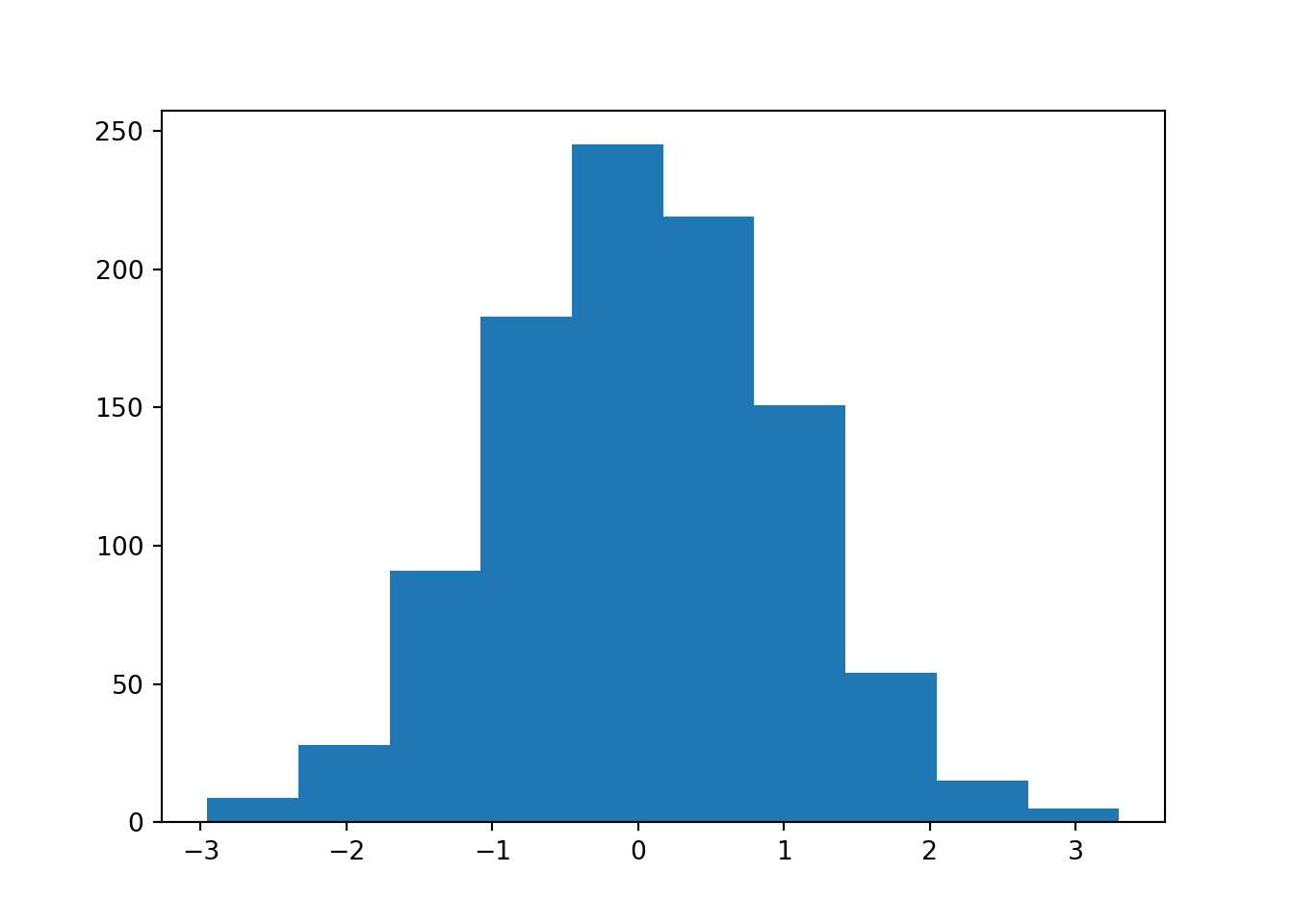
정규분포

s = np.random.normal(0, 1, 1000)

import matplotlib.pyplot as plt
plt.hist(s)

## (array([  9.,  28.,  91., 183., 245., 219., 151.,  54.,  15.,   5.]), array([-2.95437005, -2.3291265 , -1.70388296, -1.07863942, -0.45339587,
##         0.17184767,  0.79709121,  1.42233476,  2.0475783 ,  2.67282184,
##         3.29806539]), <a list of 10 Patch objects>)

plt.show()